Beyond Family Labels: A Taxonomic Ornstein–Uhlenbeck Prior for Avian 3D Shape Recovery
Abstract
Recovering 3D pose and shape of birds from single images is bottlenecked by the long tail of avian diversity: out of ~10,000 species, only a few dozen have 3D-labeled training data, and in-the-wild test sets routinely contain species never seen at training. Generalizing across clades is therefore a central problem. The current state of the art, AniMer+, mitigates it with a family-level contrastive loss that conveys only a binary same-family indicator per pair and discards the continuous structure of the species tree.
We propose a taxonomic Ornstein–Uhlenbeck prior on the shape code of the AVES parametric bird mesh model: a multivariate Gaussian whose covariance decays exponentially with Linnaean rank distance, with a learnable selection strength and noise scale. The prior generalizes family contrastive into a continuous, generative form, exposing the graded cross- and within-family similarity that a binary indicator cannot, and brings continuous comparative phylogenetics in as a biology-grounded inductive bias for the long tail.
Our method improves over AniMer+ on both metrics of the unseen-species CowBird benchmark and on CtrlAVES3D, while remaining comparable on seen-species CUB. A permutation ablation isolates taxonomic structure from generic Gaussian smoothing, and a rank-granularity ablation identifies cross-order distinctions (the structure beyond a family-vs-not indicator) as the dominant source of the unseen-species gain.
Overview
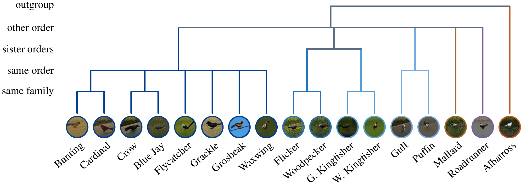
The 17 training species on the taxonomic tree. AniMer+ only asks whether two species join below the dashed red line (same family). Our prior uses every level: the closer two species are, the more strongly their shapes are tied.
Click the tree to see how it becomes the distance matrix.
Method
Click the figure for a panel-by-panel walkthrough.
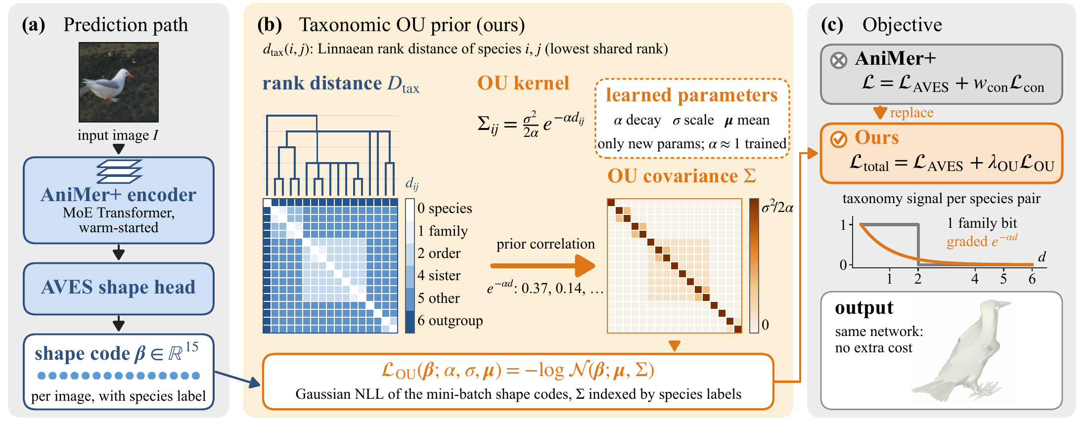
Overview. We keep the AniMer+ network (blue) and change only its training loss (orange). Closely related species tend to have similar body shapes, and the similarity fades as the relationship becomes more distant. Comparative biology models exactly this with an Ornstein–Uhlenbeck (OU) process: a trait evolving along the species tree, whose correlation between two species decays exponentially with their tree distance. We place that model as a Gaussian prior on the 15-dimensional AVES shape code β, with the distance read from standard Linnaean taxonomy, and use its negative log-likelihood in place of AniMer+’s binary family contrastive loss. The network, and its cost at test time, stay the same; the only new parameters are the two scalars α, σ and the mean μ.
Step by step
Click any step for the full explanation.
Linnaean rank distance
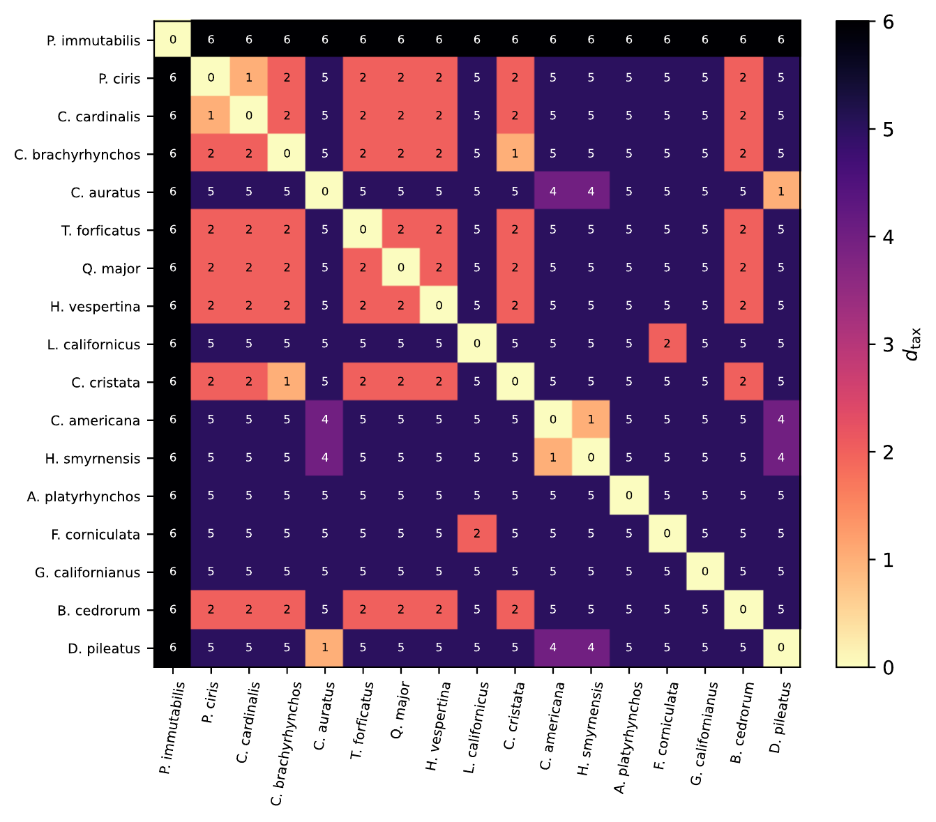
A fixed 17×17 matrix of integer ranks read off standard taxonomy: 0 same species, 1 same family, 2 same order, 4–6 across orders.
OU covariance over species
Correlation between two species’ shape codes decays exponentially with their tree distance.
Gaussian NLL on shape codes
Score each mini-batch of shape codes under the prior, with Σ indexed by their species labels.
Family contrastive is a corner case
In the α → ∞ limit the kernel reduces to family blocks, a structural analogue of AniMer+’s binary same-family view. At α ≈ 1, where training keeps it, the prior stays graded.
Drop-in replacement in AniMer+
Swap the contrastive term for the OU term. Same network at test time, so no extra cost.
How it works: a four-bird toy example
Two sparrows (one family) and two warblers (another family), all in one order. Drag α to see the covariance change; click a card for details.
Tree cut at family → 1 or 0
Same family = 1, anything else = 0.
Whole tree → covariance
Similarity decays with tree distance: e−αd.
NLL pulls codes toward relatives
Strong pull within a family, weak within an order: family neighborhoods tighten, while the tree-like layout from pre-training is kept.
Results
Keypoints move toward the ground truth
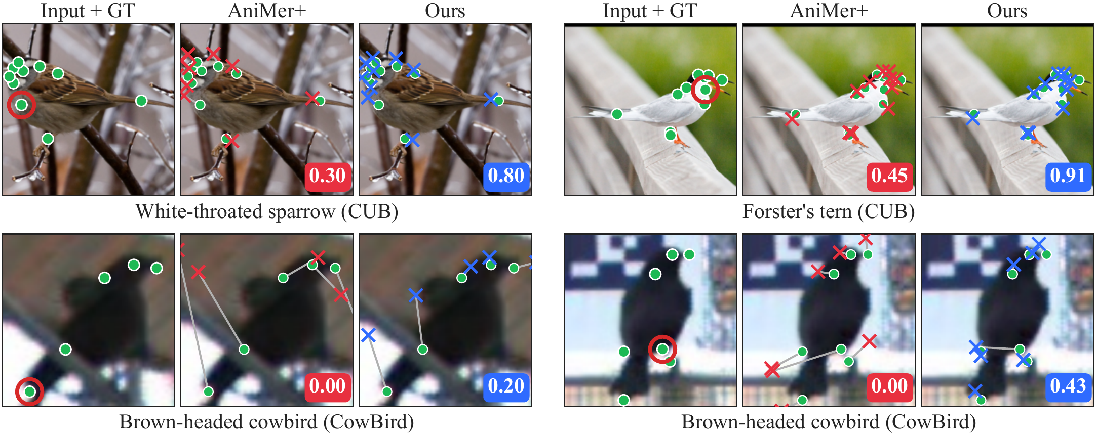
CUB (top) and CowBird (bottom). Green: ground truth · red ×: AniMer+ · blue ×: ours.
Method at a glance
(a) Prediction path: unchanged
The AniMer+ encoder (a mixture-of-experts Vision Transformer, warm-started from the released bird+mammal checkpoint) maps a single image to the parameters of AVES, a multi-species parametric bird mesh. Its shape is controlled by a 15-dimensional code \(\boldsymbol\beta\). Every training image also carries a species label.
(b) Taxonomic OU prior: what we add
Across the 17 training species, we model the shape codes as a multivariate Gaussian whose covariance is an Ornstein–Uhlenbeck kernel over a fixed Linnaean rank-distance matrix \(D_{\mathrm{tax}}\). The kernel has two learnable scalars, the decay \(\alpha\) and scale \(\sigma\), plus a learnable mean \(\boldsymbol\mu\). The negative log-likelihood of the mini-batch codes under this Gaussian is the loss \(\mathcal{L}_{\mathrm{OU}}\).
(c) Objective: one term swapped
\(\mathcal{L}_{\mathrm{OU}}\) replaces AniMer+’s family contrastive term (\(w_{\mathrm{con}} = 0\)), so on birds the loss is \(\mathcal{L}_{\mathrm{total}} = \mathcal{L}_{\mathrm{AVES}} + \lambda_{\mathrm{OU}}\,\mathcal{L}_{\mathrm{OU}}\). The lower-right plot shows the difference per species pair: AniMer+ gets one bit (same family or not), while the prior gets a graded signal \(e^{-\alpha d}\) at every rank.
Blue: the existing network and fixed taxonomy. Orange: what we add.
Linnaean rank distance \(D_{\mathrm{tax}}\)
The prior needs one number per pair of species saying how related they are. We read it straight off standard avian taxonomy (the IOC World Bird List): the lower the rank at which two species meet, the smaller their distance.
| \(d_{\mathrm{tax}}\) | Lowest shared group | Example from the 17 training species |
|---|---|---|
| 0 | same species | — |
| 1 | same family | Painted Bunting – Northern Cardinal (Cardinalidae) |
| 2 | same order | American Crow – Boat-tailed Grackle (Passeriformes) |
| 4 | sister orders | Northern Flicker – Green Kingfisher (Piciformes – Coraciiformes) |
| 5 | other orders | Mallard – California Gull |
| 6 | outgroup | Laysan Albatross – any other species |
The cross-order values (4–6) are informed by the whole-genome avian phylogeny of Jarvis et al. (2014); the values 5 and 6 are ordinal design choices. Restricted to the 17 CtrlAVES3D species, this gives a fixed, non-learnable 17×17 matrix. The species set comes with the dataset; it contains no two species of the same genus, so the genus rank never appears.
Why Linnaean ranks rather than a molecular tree?
Comparative biology usually feeds an OU kernel patristic distances, path lengths through a dated tree such as the Jetz et al. avian supertree. We use integer ranks for two reasons.
- Conditioning. On these 17 species, Jetz distances span 18.6 to 201.2 million years. For \(e^{-\alpha d}\) to give meaningful cross-family correlation on that scale, \(\alpha\) would need to sit near \(10^{-2}\), which leaves an almost diagonal covariance where our optimizer actually converges (\(\alpha \sim 1\)). Rank values \(\{1,2,4,5,6\}\) are on the same scale as the converged \(\alpha\), so species share information without any rescaling.
- Little signal lost. The ranks correlate strongly with Jetz distances on this subset (Pearson 0.85, Spearman 0.76). The Jetz tree is used only for this check and for evaluation; training sees \(D_{\mathrm{tax}}\) alone.
OU covariance over species
In comparative biology, the Ornstein–Uhlenbeck process is the standard model of a continuous trait evolving along a species tree while being pulled toward an optimum. Under it, the trait values of two species are correlated, and the correlation decays exponentially with their distance on the tree. We treat the AVES shape code as that trait.
We wanted a species-level prior that (a) places shape codes of related species near each other in \(\mathbb{R}^{15}\), (b) does so with a strength that fades smoothly with taxonomic distance instead of stopping at a hard family cut, and (c) keeps a global “how much can shape vary” knob separate from a relational “how similar are sister species” knob. The OU kernel does all three by construction.
The two knobs
- \(\alpha\): selection strength (decay rate). Large \(\alpha\) collapses the kernel to sharp, family-like blocks. Small \(\alpha\) smears similarity across the whole taxonomy. As \(\alpha \to 0\) you recover Brownian motion, where covariance is proportional to shared branch length.
- \(\sigma\): noise scale. Together with \(\alpha\) it sets the stationary variance \(\sigma^2/2\alpha\), the prior’s marginal scale for each species.
What the correlations look like at \(\alpha = 1\)
| Pair | \(d\) | \(e^{-\alpha d}\) |
|---|---|---|
| same family | 1 | 0.37 |
| same order | 2 | 0.14 |
| sister orders | 4 | 0.018 |
| other orders | 5 | 0.0067 |
| outgroup | 6 | 0.0025 |
A graded ladder, not a single on/off switch. The toy example on the page lets you drag \(\alpha\) and watch the matrix change.
Implementation: \(\alpha\) and \(\sigma\) are kept positive with a softplus (floor \(\alpha_{\min} = 10^{-3}\)) and initialized at \(\alpha_0 = \sigma_0 = 1\).
Gaussian NLL on mini-batch shape codes
For a mini-batch of \(B\) images with species labels \(s_1,\dots,s_B\), the encoder predicts shape codes \(\boldsymbol\beta \in \mathbb{R}^{B\times D}\) (\(D = 15\)). We index the OU kernel with those labels to get a \(B\times B\) covariance, then score the codes under that Gaussian.
Each of the 15 shape dimensions is treated as an independent sample that shares the same species covariance.
Reading the two terms
- Quadratic (Mahalanobis) term. \(\Sigma^{-1}\) couples the instances in the batch. Two images of closely related species are penalized for disagreeing on their codes: strongly within a family, weakly within an order, and hardly at all across distant orders. This is the “pull toward relatives”.
- Log-determinant term. It does not depend on the codes, only on \((\alpha, \sigma)\) and on which species are in the batch. As usual for a Gaussian NLL, it balances the quadratic term: \((\alpha, \sigma)\) cannot shrink the loss just by inflating the variance.
- Learnable mean \(\boldsymbol\mu \in \mathbb{R}^{15}\). A single learned mean, shared by all species, so the prior pulls codes toward a learned center rather than a fixed origin.
Why a likelihood, not a metric-learning loss?
The NLL gives the prior a generative reading: the same \(\Sigma\) in the loss is a Gaussian-process covariance, which the supplementary material uses for a MAP interpretation. It also makes the comparison with family contrastive clean in the \(\alpha\to\infty\) limit (Step 4).
Family contrastive is the \(\alpha \to \infty\) corner
AniMer+ uses a family-level supervised contrastive loss: same-family pairs are pulled together and every other pair is pushed apart. That is one bit of taxonomy per pair. Our prior contains a structural analogue of this view as a limiting case, and goes beyond it.
The limit
Use a block convention in which same-family pairs sit at distance 0 and everything else at distance > 0 (our actual \(D_{\mathrm{tax}}\) puts same family at 1, so this is a shifted version), and let \(\alpha \to \infty\) while holding the stationary variance \(\sigma^2/2\alpha\) fixed. Every off-family correlation goes to zero and the kernel collapses to a family-indicator block matrix. That prior pulls same-family codes toward a shared family mean and leaves different families uncorrelated, which is the same qualitative effect contrastive learning has in feature space. In this sense \(\mathcal{L}_{\mathrm{OU}}\) is a Gaussian, probabilistic relaxation of the binary same-family indicator.
The analogy is structural, not literal
- Singular covariance. At the limit the block matrix is rank-deficient, so the strict Gaussian NLL is undefined; it needs jitter and a pseudo-inverse, with the limit analyzed as \(\varepsilon \to 0\).
- Different representations. Contrastive learning works on \(L_2\)-normalized class-token features with a cosine-softmax objective. \(\mathcal{L}_{\mathrm{OU}}\) works on raw shape codes \(\boldsymbol\beta \in \mathbb{R}^{15}\) through a quadratic form. They are best read as analogous regularizers on different representations.
Why it matters
Training keeps \(\alpha\) finite, near its initial value of 1, not infinity. There the correlations form a graded ladder down the hierarchy (see the table in Step 2). That graded structure is exactly what a family-vs-not indicator cannot represent. The rank-granularity ablation tests this directly: its family-only matrix plays the role of this corner.
A drop-in change to AniMer+
The network is untouched; only the training loss changes.
\(\mathcal{L}_{\mathrm{AVES}}\) holds the keypoint, silhouette and shape/pose regression terms for birds; the mammal branch \(\mathcal{L}_{\mathrm{SMAL}}\) is inactive in our bird-only setting. \(f_{\mathrm{batch}}\) is the species index of each sample. With \(w_{\mathrm{con}} = 0\), the OU prior is the only taxonomy-aware regularizer.
Properties
- Exact nesting. Restore \(w_{\mathrm{con}}\) and set \(\lambda_{\mathrm{OU}} = 0\), and you get the AniMer+ training loop back to floating-point equality. The OU contribution is isolated in one hyperparameter.
- No inference cost. The only new parameters are \(\alpha\), \(\sigma\) and \(\boldsymbol\mu\), and they are used only by the loss. At test time it is the same network.
- Separate learning rate. \((\alpha, \sigma, \boldsymbol\mu)\) sit in their own AdamW group, at \(k\times\) the backbone learning rate (\(k = 100\) in all headline runs). Results barely change across \(k \in \{1, 10, 30\}\). So the gain comes primarily from the shape of the regularizer at its initialization \((\alpha_0, \sigma_0) = (1, 1)\). Fitting the scalars is a secondary effect: only at \(k = 100\) does it shift CowBird PCK, by about +1 pt.
Setup
What the prior does in shape space
During training, the NLL pulls each shape code toward the codes of related species, with a strength set by \(\Sigma\): strong within a family, weak within an order, almost none across distant orders.
The pre-trained model’s shape codes already place related species close together. The prior does not create that tree-like layout; it keeps it and tightens each family’s neighborhood. The unseen-species gain on CowBird is consistent with cross-species borrowing. But real and shuffled trees produce similar code geometry, so the difference between them likely lives in the encoder rather than in the codes themselves.
What we actually measure
- The share of each code’s 10 nearest neighbors that belong to its family rises from 0.61 → 0.68 (headline strength) → 0.73 (\(\lambda_{\mathrm{OU}} = 10^{-4}\)).
- All 136 species pairs move closer (0.85× on average), but their order is nearly unchanged (Spearman 0.99). The prior tightens the space; it does not rearrange it.
Keypoints move toward the ground truth
Two CUB-200 test images (top) and two CowBird instances (bottom) of the Brown-headed Cowbird, a species seen at neither training stage, chosen as cases where the baseline misplaces several keypoints. For a fair comparison, the baseline is AniMer+ retrained with its published recipe for the same 30,000 steps.
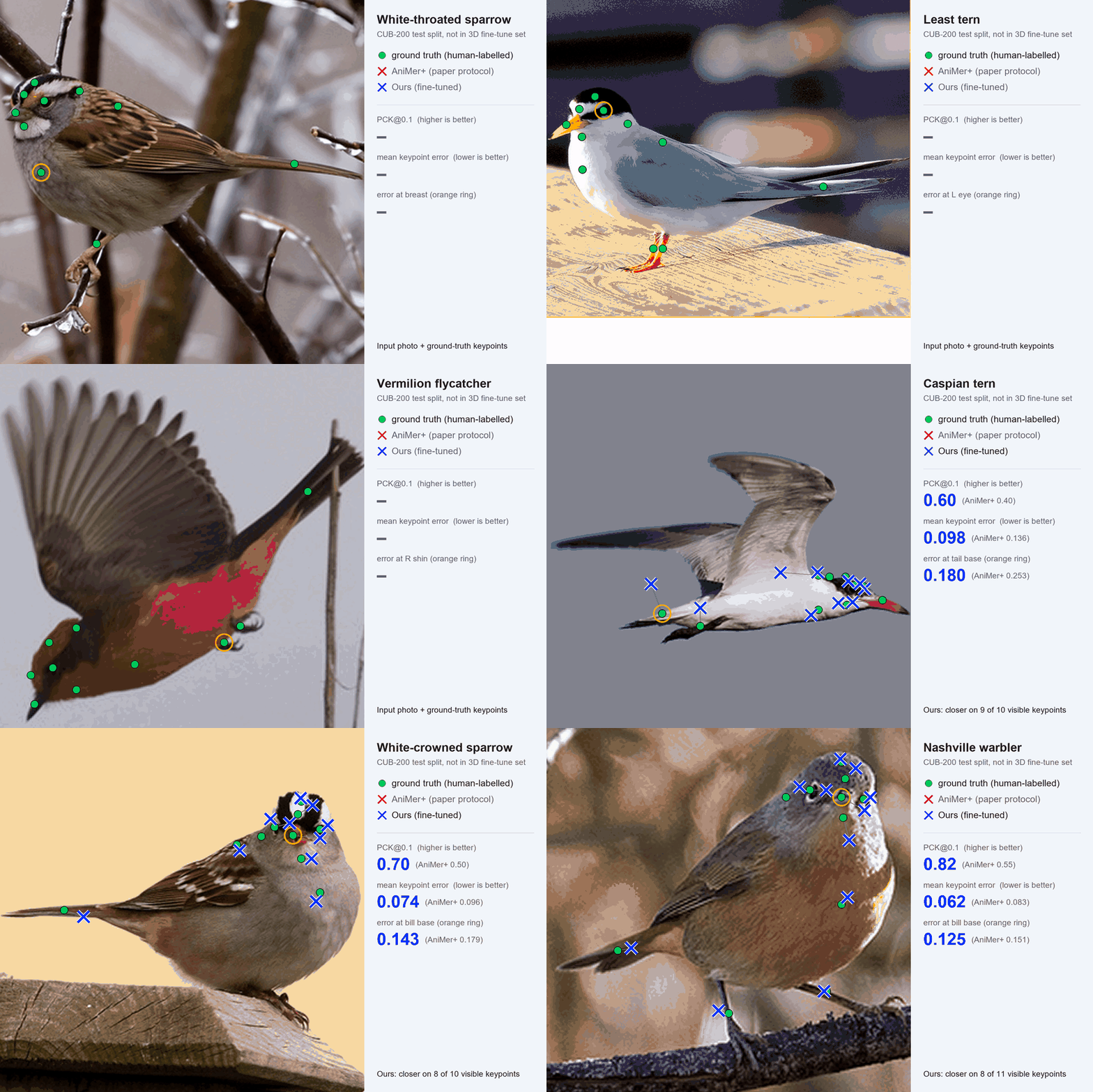
In all four cases the OU fine-tune moves the keypoint set toward the ground truth. More paired examples are in the supplementary material, and the animation at the top of the page shows eight more CUB species from outside the 17-species fine-tuning set.
These are selected cases, not a statistical sample: they show the kind of correction the fine-tune makes, not how often it makes one.
These examples are illustrative. The numbers to rely on are in the main table.
The gain is on unseen species
Against AniMer+, the prior improves both metrics on the unseen-species CowBird benchmark, by +1.5 AUC and +2.5 PCK@0.1. On CtrlAVES3D it is on par (93.05 vs. 93.00 AUC), and on seen-species CUB it is comparable.
Benchmarks
- CUB-200-2011: seen-species fine keypoint localization. All 200 CUB species are in AniMer+ pre-training, so they count as seen even though only 17 are in our fine-tuning set.
- CowBird: the unseen-species, out-of-distribution test. It covers a single species, the Brown-headed Cowbird, which appears in neither AniMer+ pre-training nor our fine-tuning. This is where borrowing shape from relatives should help most, and where the gain is concentrated.
- CtrlAVES3D test split: 3D reconstruction on the 17 training species.
Metrics
PCK@0.1 is the fraction of predicted 2D keypoints within a normalized distance of 0.1 from the ground truth. AUC is the area under the PCK curve as the threshold sweeps from 0 to 1. Higher is better for both.
Reading the table
- Ours is the mean ± sample standard deviation over five seeds. The standard deviations (≤ 0.27) are small compared with the CowBird gains.
- AVES and HMR2.0 are the baselines reported by AniMer+.
- AniMer-A is a bird-only specialist that gives up AniMer+’s unified bird+mammal coverage. The like-for-like comparison is ours vs. the unified AniMer+.
- On CUB the prior gives up a little seen-species precision (89.30 vs. 89.50 AUC). This is consistent with the seen/unseen trade-off in the rank ablation. Note that the AniMer+ row is its paper-reported number, not a run from our pipeline.
Training: fine-tuned from the released AniMer+ checkpoint on the 6,464-image CtrlAVES3D train split for 30,000 steps, \(\lambda_{\mathrm{OU}} = 10^{-5}\), cosine schedule. Evaluation follows the AniMer+ protocol.
The gain comes from the real tree
Any regularizer that adds structure to the shape codes, even random structure, might help out-of-distribution. That would not be evidence for taxonomy. So we keep everything fixed and change only which distance matrix the OU kernel sees.
The control
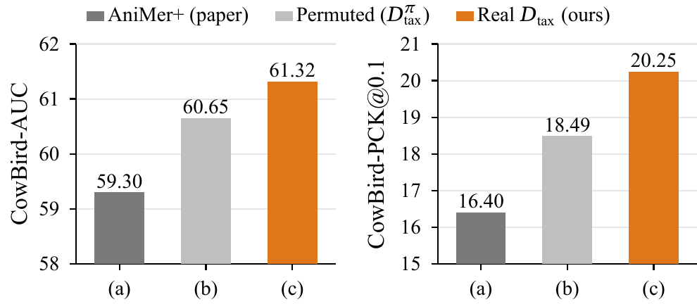
The permuted matrix shuffles which species sits where in the taxonomy. It keeps the OU kernel’s spectrum exactly, with the same covariance eigenvalues, so it is the same amount of “Gaussian smoothing”. What it destroys is the link between species labels and their true relatives.
What it shows
The real tree wins on both metrics. The prior uses which species are which, not just the fact that an OU kernel was applied. The same real-vs-permuted contrast also holds on the 183 CUB species outside the fine-tuning taxonomy, with species-clustered confidence intervals that exclude zero.
Both OU runs use the stronger ablation setting (\(\lambda_{\mathrm{OU}} = 10^{-4}\), constant learning rate) so the taxonomic signal is strong enough to see. The AniMer+ bar is the value from its paper, not a run from our pipeline; it is shown for context, not as a controlled comparison.
Ranks above the family carry most of the gain
How much of the unseen-species gain needs information beyond a family-vs-not indicator? We train with progressively richer distance matrices, all with the same configuration as the permutation ablation.
| \(D_{\mathrm{tax}}\) variant | values | CUB AUC | CUB PCK | CowBird AUC | CowBird PCK | CtrlAVES3D AUC |
|---|---|---|---|---|---|---|
| permuted (null) | — | 88.87 | 54.90 | 60.65 | 18.49 | 92.95 |
| family-only | {0,1,5} | 89.09 | 56.35 | 60.84 | 19.09 | 93.06 |
| order-only | {0,1,2,5} | 89.10 | 56.42 | 60.81 | 19.20 | 93.07 |
| Linnaean (full, ours) | {0,1,2,4,5,6} | 88.92 | 55.16 | 61.32 | 20.25 | 92.99 |
All three kernels use 0 for the same species and 1 for the same family, and differ only above the family level. The family-only and order-only kernels share a single cross-order value (5), so only the rank granularity changes, not the cross-order distance scale. The family-only kernel is the discrete analogue of the \(\alpha \to \infty\) / family-contrastive corner (Step 4).
Cross-order ranks carry the unseen-species gain
Relative to the permuted null, ranks above the family account for about 66% of the CowBird PCK improvement, and cross-order ranks alone for about 60%. Separating, say, the duck order Anseriformes from the woodpecker order Piciformes is exactly what a family-vs-not indicator cannot express. Hence the title, Beyond Family Labels.
A seen vs. unseen trade-off
On CUB PCK the pattern reverses: the coarser kernels keep more seen-species precision. Finer cross-order structure increases sharing across species. That helps unseen species at a small cost in fine localization on seen ones. The pattern is consistent with cross-species borrowing.
BibTeX
@inproceedings{jeon2026beyond,
  title     = {Beyond Family Labels: A Taxonomic Ornstein--Uhlenbeck Prior for Avian 3D Shape Recovery},
  author    = {Jeon, Yunchan and Kim, SooGon and Kim, Seungwook and Lee, CheolWon and Lee, Jongmin},
  booktitle = {Advances in Neural Information Processing Systems (NeurIPS)},
  year      = {2026}
}